This page describes the analysis model, equations, numerical steps, load handling, result recovery, and the analytical benchmarks run by the same Python solver used by the workspace.
Members use linear-elastic material behavior and small-displacement kinematics. Each member can have its own Young’s modulus E, shear modulus G, area A, second moment of area I, and effective shear area Av. The steel section database supplies the in-plane area and inertia for its profiles; concrete input is currently a rectangular gross section for elastic analysis.
Coordinate and sign conventionGlobal X is positive to the right and global Y positive upward, so gravity loads are negative in Y. Axial force is positive in tension and negative in compression. Bending moment is positive when it makes the member sag (tension on the underside of a horizontal beam) and negative when it makes it hog; the signed colours and diagram labels in the workspace follow the same rule. The steel design adapter maps the 2D in-plane moment to the major-axis bending input and sets the unavailable weak-axis moment to zero.
02 · MEMBER FORMULATION
Frame element stiffness
The backend builds a two-node, six-degree-of-freedom local stiffness matrix. Its axial block is the standard bar stiffness; bending couples the two transverse translations and end rotations.
AXIAL STIFFNESS
ka = EA / L
Resists extension and shortening along the member centreline.
SHEAR FLEXIBILITY
φ = 12EI / (GAvL2)
Used when the Include shear deformation option is on. The effective area Av comes from the section rule or the member’s manual value.
Local stiffness matrix in matrix form
Using local degree-of-freedom order \(\mathbf d_l=[u_1,v_1,\theta_1,u_2,v_2,\theta_2]^T\), the assembled element matrix is:
For member angle \(\alpha\), with \(c=\cos\alpha\), \(s=\sin\alpha\), transform the local matrix using \(\mathbf{k}_g=\mathbf{T}^T\mathbf{k}_l\mathbf{T}\):
When it is enabled, the bending coefficients are modified using the shear-flexibility parameter:
Y₁ = 12EI/[(1+φ)L³] · Y₂ = 6EI/[(1+φ)L²]Y₃ = (4+φ)EI/[(1+φ)L] · Y₄ = (2−φ)EI/[(1+φ)L]The transverse displacement recovery also includes the shear contribution V/(GAv).
This is a shear-flexible two-node frame element. For a slender member φ tends to zero and the response approaches the Euler–Bernoulli result. Rolled I/H sections use an effective web shear area derived from section dimensions; manual and rectangular concrete sections default to 5A/6 and can use the member-table value.
Figure. The shear parameter Φ = 12EI/(GAvL²) measures how much the cross-section lags behind the slope of the axis. Φ → 0 recovers the Euler–Bernoulli beam; deep or short members have a larger Φ and deflect more.
Member discretizationEach drawn member is one two-node finite element in the stiffness model. The many stations used to draw smooth response and mode-shape curves are post-processing points; they do not add elements or degrees of freedom. Split members and add nodes where the model needs a finer stiffness discretization, a property change, or an actual connection/restraint.
Truss membersAn axial-only truss member keeps only the axial term EA/L and has no end moments, so loads must act at its nodes (member loads on a truss member are transferred to its end nodes). A truss node has no rotational stiffness of its own, which is why a node that joins only truss members needs no rotational restraint. Use frame members wherever bending matters.
03 · STRUCTURAL SYSTEM
Coordinates, releases, and global solve
Local axes. For each member, its end coordinates define length L and direction cosines c and s. A transformation matrix converts nodal displacements and actions between global and local axes.
Global stiffness. Each member matrix is transformed as Ke = TT ke T and added into the global rows and columns corresponding to its two nodes.
End releases. A released member-end rotation is eliminated by static condensation. For active and released coordinates, the reduced stiffness is Kaa − KarKrr−1Kra. The compatible member load is condensed as well.
Supports. Prescribed degrees of freedom are removed from the free solve. A rotated support first transforms its translational coordinates into the support’s local axes; the selected local restraints are then enforced.
Sparse linear solve. The assembled system is stored as a sparse matrix and solved for free displacements using SciPy’s sparse direct solver:
Kff df = Pfglobal equilibrium of the unknown free degrees of freedom
After solving, the nodal displacement vector is transformed back to global coordinates. Reactions are recovered from the residual R = Kd − P at restrained degrees of freedom.
04 · ACTIONS AND POST-PROCESSING
Loads, combinations, and response recovery
Nodal forces and moments are entered directly. Member loads support uniform loads and internal point loads, each in global X or global Y. Both types can be applied to the same member at once, and multiple point loads can be placed at different distances from the member’s i-end. Member loads are converted to consistent equivalent nodal loads so they act through the same assembled equilibrium system as nodal loads.
For each solved case, the backend recovers local axial force N, shear V, bending moment M, and longitudinal/transverse displacement along each member. Distributed-load equilibrium contributes continuously along the member; point-load jumps are treated on the appropriate side of each load position. Station points also include candidate locations for interior response extrema so plotted peak values do not depend only on coarse sampling.
Load combinations are computed by linear superposition of the solved load cases. This is consistent with the model’s linear-elastic stiffness assumption. The program does not re-solve a nonlinear structural state for a combination.
Judgement: combinations and envelopesSuperposition is exact only while the structure behaves linearly, so it must not be used where supports lift off, members go slack, or second-order effects matter. The partial factors and combination rules are inputs you choose from the applicable code and National Annex; FaxinaX applies them but does not decide which combinations govern. Review every combination that can produce the maximum and the minimum of the quantity you design for, because the governing case for moment, shear, deflection and reaction is often different.
Why member point loads are separate from nodal loadsA point load placed between member ends is converted using the member interpolation functions. It does not require creating a node at the load location. Uniform and point loads may coexist, including in different global directions.
05 · VIBRATION ANALYSIS
Modal analysis and mass source
Choose Modal analysis in the Results overview, click Run analysis, then select a load case or combination as a mass source. The eigenvalue solver uses the same elastic frame stiffness, support rotations, member releases, and shear-deformation setting as static analysis.
Kff φ = ω² Mff φgeneralized eigenproblem on the unrestrained degrees of freedom · f = ω/(2π) · T = 1/f
Member self-mass follows the consistent two-node frame mass matrix, based on each member’s density ρ and area A. In local coordinates, the matrix is (ρAL/420) times a dimensioned 6×6 coefficient matrix; it includes axial translation, transverse translation, and rotational coupling. It is transformed into global coordinates and assembled over all members. The sparse symmetric generalized eigenproblem returns the lowest requested positive modes.
Convert selected loads into translational mass
Mass conversion is optional in global X and global Y independently. For a selected case, or each nonzero case in a selected combination, the app converts the absolute factored force magnitude by:
m = |γF| / g with g = 9.80665 m/s²γ is the load-combination factor; for a single load case γ = 1.
A nodal force becomes mass at that node’s matching global translation degree of freedom.
A uniform member load contributes |w|L/g, split equally between the two end nodes in the chosen global direction.
An internal member point load contributes |P|/g, apportioned between end nodes according to its relative position along the member.
Moments do not become translational mass; unchecked directions are ignored. For a combination, absolute factored load contributions accumulate, so opposing signs do not cancel mass.
Interpretation of mode shapesDisplayed mode shapes are normalized so the maximum member centerline displacement is 1 m for plotting convenience. Their amplitude is arbitrary; it is not a predicted vibration amplitude or static deflection. The modal solver currently includes elastic member stiffness and mass, but no damping, geometric stiffness, or forced-vibration time history.
Quick sanity check of a frequencyFor a simply supported uniform beam with mass per unit length μ, f1 = (π / 2L²)·√(EI/μ). For a cantilever, f1 = (1.875² / 2πL²)·√(EI/μ) ≈ 0.56·√(EI/μ)/L². A frame is stiffer than a free cantilever and softer than a fully fixed beam, so its first frequency should fall between simple bounds like these. A frequency far outside them usually means wrong units, a missing mass source, or a missing or extra release. The cause is rarely the eigenvalue solver.
06 · SEISMIC ANALYSIS
Modal response spectrum
The X-direction spectrum analysis uses natural periods and mode shapes from modal analysis. For influence vector \(\mathbf r_x\), each mode has participation factor \(\Gamma_n\) and effective modal mass \(M_n^*\):
The modal displacement contribution is \(\mathbf u_n=\boldsymbol{\phi}_n\Gamma_nS_a(T_n)/\omega_n^2\). Modal results are combined using SRSS or CQC. Since a response-spectrum result is an envelope magnitude, plotted signs follow the dominant modal contribution.
EN 1998-1:2004/2005 design spectrum
For the EN 1998-1 design spectrum, \(a_g=\gamma_Ia_{gR}\). The ground type and spectrum type define \(S,T_B,T_C,T_D\):
The lower bound \(\beta a_g\) applies on the descending branches. Modal force response uses \(S_d(T)\); modal displacement includes the behaviour-factor scaling defined by the analysis procedure.
EN 1998-1-1:2024 elastic response spectrum
The 2024 formulation uses mapped reference spectral accelerations (S_{\alpha,RP}) and (S_{\beta,RP}), site factors (F_\alpha) and (F_\beta), and the topographic factor (F_T). The zero-period ratio (F_A) is a separate parameter:
Here \(\xi\) is the damping ratio in percent. The standard NDP defaults shown in the tool are \(T_A=0.02\,\mathrm{s}\), \(F_A=2.5\), and \(\chi=4\). The default \(T_D\) depends on \(S_{\beta,RP}\). Supply project-specific mapped hazard, site, and National Annex parameters. If \(T_C\ge1\,\mathrm{s}\), the NDP calls for a spectrum-specific study.
EN 1998-1-1:2024 reduced spectrum for force analysis
The force-based approach reduces the elastic spectrum using \(q=q_Rq_Sq_D\). The reduction is period dependent below \(T_B\):
Force and displacement responseThe lower bound \(\beta S_{\alpha,RP}(T)\) applies to force calculations. It is excluded from displacement recovery. For design-spectrum displacement, the first-mode displacement behaviour factor is \(q_{disp}=q\) when \(T_1\ge T_B\), otherwise \(q_{disp}=\min\{3q,\,1+(q-1)T_B/T_1\}\).
The 2024 elastic displacement spectrum transforms acceleration for shorter periods and extends the curve at long periods:
When \(v_{s,H}\) is available, \(F_L=(v_{s,H}/800)^{-0.4}\). Otherwise the site-category default for \(F_L\) is used. For reduced-spectrum design, the tool scales modal displacement with \(q_{disp}\), while the force spectrum lower bound does not enter the displacement calculation.
Reduced spectrum in this toolNamed “Reduced spectrum” in the 2024 design option. It uses the user-provided mapped hazard and site inputs and applies the lower bound only to modal force response.
For CQC, \(\rho_{ij}\) depends on modal frequency ratio and viscous damping. The 2024 edition uses a distinct single-spectrum hazard parameterization and reduced spectrum; Type 1 and Type 2 apply to the earlier edition. Use project-specific hazard and National Annex parameters. See the BSI EN 1998-1-1:2024 publication page.
Judgement: using spectrum resultsInclude enough modes so that the effective modal masses in the analysed direction add up to at least 90 % of the total mass (EN 1998-1 also accepts all modes with more than 5 % effective mass). The spectrum analysis here is for the global X direction of a 2D model; it does not include accidental torsion, vertical action or a second horizontal direction. SRSS and CQC give magnitudes without a reliable sign, so when you combine a seismic action with gravity loads, check both signs of the seismic effect. Judge whether the behaviour factor q is justified by the structure’s ductility and detailing: the solver cannot assess it.
07 · ANALYTICAL VALIDATION
Verification examples
Three benchmark models were run through the production analysis function. Selected reactions, moments and displacement are compared below with closed-form solutions, and global static equilibrium is evaluated for each model. The benchmarks use E = 210 GPa, I = 8×10⁻⁵ m⁴, L = 6 m, and disable shear deformation so the comparison matches classical beam formulas.
A
Propped cantilever · flexibility method
One member carries q = 10 kN/m downward and P = 20 kN downward at midspan. The free cantilever end displacement is set to zero by the prop reaction.
RB = 3qL/8 + 5P/16 = 28.75 kN
RA = qL + P − RB = 51.25 kN; |MA| = 67.50 kNm
B
Fixed-fixed beam · slope-deflection
A fixed-ended member carries a uniform load q = 10 kN/m downward. With no sidesway, the slope-deflection equations are MAB = MABF + (2EI/L)(2θA + θB) and MBA = MBAF + (2EI/L)(2θB + θA). Fixed joints set θA = θB = 0, so the uniform-load fixed-end moment magnitudes are qL²/12. Global equilibrium gives the two vertical reactions.
|MAB| = |MBA| = qL²/12 = 30.00 kNm
RA = RB = qL/2 = 30.00 kN
C
Simply supported beam · internal point load
A 10 kN point load is placed at midspan inside one member, with no interior node. This checks the member point-load interpolation and the exact elastic beam response.
RA = RB = P/2 = 5.00 kN; Mmax = PL/4 = 15.00 kNm
|δmid| = PL³/(48EI) = 2.67857 mm
Verification run on 29 October 2026 with the production FaxinaX solver: all 11 response comparisons and all 3 global-equilibrium checks passed. Tolerance: relative error ≤ 1×10⁻⁷, equilibrium residual ≤ 1×10⁻⁷ kN or kNm.
CASE A · VERIFIED
Propped cantilever · flexibility method · member point load plus uniform load
PASS
The prop reaction is the redundant. At the prop, the total elastic deflection is zero. Superposition of the cantilever deflections gives RB = 3qL/8 + 5P/16 for a midpoint point load, then vertical force and moment equilibrium give the fixed-end reactions.
Quantity
Analytical
FaxinaX
Difference
Relative error
Status
left vertical reaction
51.250000 kN
51.250000 kN
0
0.00000000 %
PASS
prop vertical reaction
28.750000 kN
28.750000 kN
0
0.00000000 %
PASS
fixed-end moment magnitude
67.500000 kNm
67.500000 kNm
0
0.00000000 %
PASS
Global equilibrium residualsΣFx 0.0000000000 kNΣFy 0.0000000000 kNΣMz 0.0000000000 kNmEQUILIBRIUM PASS
With zero joint rotations and no sidesway, slope-deflection gives |MAB| = |MBA| = qL²/12. Static equilibrium then gives vertical reactions qL/2 at each end.
Quantity
Analytical
FaxinaX
Difference
Relative error
Status
left vertical reaction
30.000000 kN
30.000000 kN
0
0.00000000 %
PASS
right vertical reaction
30.000000 kN
30.000000 kN
0
0.00000000 %
PASS
left end moment magnitude
30.000000 kNm
30.000000 kNm
0
0.00000000 %
PASS
right end moment magnitude
30.000000 kNm
30.000000 kNm
0
0.00000000 %
PASS
Global equilibrium residualsΣFx 0.0000000000 kNΣFy 0.0000000000 kNΣMz 0.0000000000 kNmEQUILIBRIUM PASS
CASE C · VERIFIED
Simply supported beam · internal member point load · exact elastic solution
PASS
The 10 kN point load acts at midspan inside a single member, separately from nodal loads. Symmetry gives 5 kN at each support and Mmax = PL/4. Euler-Bernoulli midspan deflection is PL³/(48EI).
Quantity
Analytical
FaxinaX
Difference
Relative error
Status
left reaction
5.000000 kN
5.000000 kN
0
0.00000000 %
PASS
right reaction
5.000000 kN
5.000000 kN
0
0.00000000 %
PASS
maximum bending moment magnitude
15.000000 kNm
15.000000 kNm
0
0.00000000 %
PASS
midspan deflection magnitude
2.678571 mm
2.678571 mm
0
0.00000000 %
PASS
Global equilibrium residualsΣFx 0.0000000000 kNΣFy 0.0000000000 kNΣMz 0.0000000000 kNmEQUILIBRIUM PASS
Pass criterion: each listed response has relative error ≤ 1×10⁻⁷, and the absolute global force and moment residuals are each ≤ 1×10⁻⁷ kN or kNm. The results above are a recorded run; they are repeated whenever the solver changes. These are idealized benchmark checks, not proof that every possible model, support arrangement, or load case is error-free.
Checks that run on your own modelThe benchmarks above test the solver on fixed examples. For your own model, every run also performs a Result check: it looks for a mechanism and names the cause (too few supports, supports that cannot stop rigid-body motion, or too many releases), isolated nodes and disconnected parts, huge displacements, deflection above span/50, and values that suggest wrong units. It also verifies global equilibrium for each load case and combination: the support reactions must equal the applied loads, including self-weight (ΣFx, ΣFy and ΣM). For a pure self-weight case the total vertical reaction must equal the total weight of the members. These checks catch modelling mistakes. They cannot show that the model represents the real structure.
08 · BRIDGE TRUSS CASE STUDY
Independent verification of a truss bridge
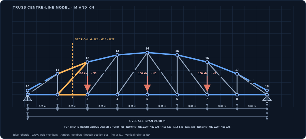
This worked example uses the same centre-line topology as the supplied bridge model. It compares FaxinaX static analysis with independent equilibrium calculations: support reactions from whole-structure statics, member forces from joints and a section cut, and nodal deflections from the virtual-work method.
18nodes
33axial members
8 × 3.01 mpanels · 24.08 m span
4.45 mmaximum height
1. Centre-line model and dimensions
The lower chord lies at y = 0. Nodes 1–9 are spaced every 3.01 m from x = 0 to 24.08 m. Nodes 10–18 share those horizontal coordinates; their elevations are 0.45, 2.20, 3.45, 4.20, 4.45, 4.20, 3.45, 2.20, and 0.45 m.
Coordinates and member connectivity follow bridge-models/middle-road-truss.json. Amber members cross section I–I. Dimensions are in metres.
Supports and idealization
Node 1 is pinned: ux = uy = 0.
Node 9 is a vertical roller: uy = 0; horizontal movement is free.
Members are pin-jointed, axial-only truss elements; self-weight and member loads are excluded.
All members use the sample model’s assumed 600 × 900 mm concrete section, A = 0.540 m², and E = 32.836568 GPa (C30/37). These assumed values are for this verification example, not a bridge design recommendation.
Applied nodal load case
Three vertical point loads act downward at lower-chord nodes 3, 5, and 7:
N3 100 kNN5 150 kNN7 100 kN
Total applied load = 350 kN. No horizontal loads or applied moments.
2. Static analysis: reactions and member forces
Taking moments about the left support and then summing vertical forces gives the reactions. There is no applied horizontal load, so the pin’s horizontal reaction is zero.
At node 1, M1 runs horizontally to node 2 and M26 runs to node 11. Unloaded joint 10 first gives M9 = M17 = 0. The known force at node 1 is its 175 kN upward reaction. M26 has direction cosines (0.807342, 0.590084). Taking tension as positive:
Free-body diagram after resolving the unloaded joint N10. The blue arrow shows the support reaction, the green arrow is the positive-tension assumption for M1, and the red arrow shows the actual compressive force in M26.
Repeating joint equilibrium across the determinate truss gives the axial force in every member. Positive values indicate tension (T); negative values indicate compression (C).
The calculation log below exposes the sequence instead of reporting only final member forces. For every joint it shows the already-known force resultant, the member force unknowns, each scalar equilibrium equation using the member direction cosines, and the solved tension-positive axial forces.
Joint-by-joint equilibrium log · all 18 joints
Tension is positive. Each row lists the known force resultant at that joint (external loads, support reaction, and previously solved bars). Direction cosines are resolved from the listed node coordinates. The two scalar equilibrium equations are then solved for the currently unknown bar forces. Rows follow a valid solve order; zero-force members at unloaded joints are identified first.
All incident members are known; ΣFx = 0 and ΣFy = 0.
Equilibrium satisfied
Method of sections: independent cut check
Section I–I cuts members M2, M10, and M27. Isolating the left-hand part and taking moments about node 1 eliminates the force in M2 because its line of action passes through that node. The three equilibrium equations are:
The section cut therefore gives M2 in tension and M10 and M27 in compression. No point load lies to the left of this cut, so these values are unchanged by moving the loads to nodes 3, 5, and 7.
3. Analytical displacement by virtual work
For a truss, the displacement in a chosen direction follows from axial strain energy. Apply a unit downward force at the target node to obtain virtual member forces ni; combine them with actual member forces Ni:
For each target displacement, apply a unit downward force at that node and solve the virtual truss. With the three applied loads at N3, N5, and N7, the virtual-work results are 1.140831 mm downward at N3, 1.601666 mm downward at N5, and 1.140831 mm downward at N7.
4. Compare hand calculations with the Python solver
Result
Analytical method
FaxinaX static
Agreement
Reaction at node 1, R1y
175.000 kN
175.000 kN
Matches
Reaction at node 9, R9y
175.000 kN
175.000 kN
Matches
Member M1, N1
+239.432 kN (T)
+239.432 kN (T)
Matches
Member M26, N26
−296.568 kN (C)
−296.568 kN (C)
Matches
Member M2, N2
+305.362 kN (T)
+305.362 kN (T)
Matches
Member M10, N10
−259.257 kN (C)
−259.257 kN (C)
Matches
Member M27, N27
−100.286 kN (C)
−100.286 kN (C)
Matches
Node 3 vertical deflection
−1.140831 mm
−1.140831 mm
Matches
Node 5 vertical deflection
−1.601666 mm
−1.601666 mm
Matches
Node 7 vertical deflection
−1.140831 mm
−1.140831 mm
Matches
The independent joint-equilibrium solution was compared against the production api.analyze() solver for all 33 members. Maximum absolute axial-force difference: 1.14e-12 kN; maximum vertical reaction difference: 4.55e-13 kN. Virtual-work and FE displacements agree within numerical round-off at N3, N5, and N7.
Show all 33 member axial forces: method of joints versus FE solver
Member
Connectivity
Joints / sections (kN)
FE solver (kN)
State
M1
1–2
239.432
239.432
Tension
M2
2–3
305.362
305.362
Tension
M3
3–4
304.583
304.583
Tension
M4
4–5
338.202
338.202
Tension
M5
5–6
338.202
338.202
Tension
M6
6–7
304.583
304.583
Tension
M7
7–8
305.362
305.362
Tension
M8
8–9
239.432
239.432
Tension
M9
10–11
0.000
0.000
Zero-force
M10
11–12
−259.257
−259.257
Compression
M11
12–13
−314.699
−314.699
Compression
M12
13–14
−305.632
−305.632
Compression
M13
14–15
−305.632
−305.632
Compression
M14
15–16
−314.699
−314.699
Compression
M15
16–17
−259.257
−259.257
Compression
M16
17–18
0.000
0.000
Zero-force
M17
1–10
0.000
0.000
Zero-force
M18
2–11
75.568
75.568
Tension
M19
3–12
+98.913
+98.913
Tension
M20
4–13
49.702
49.702
Tension
M21
5–14
+150.000
+150.000
Tension
M22
6–15
49.702
49.702
Tension
M23
7–16
+98.913
+98.913
Tension
M24
8–17
75.568
75.568
Tension
M25
9–18
0.000
0.000
Zero-force
M26
1–11
−296.568
−296.568
Compression
M27
2–12
−100.286
−100.286
Compression
M28
3–13
1.337
1.337
Tension
M29
4–14
−60.005
−60.005
Compression
M30
6–14
−60.005
−60.005
Compression
M31
7–15
1.337
1.337
Tension
M32
8–16
−100.286
−100.286
Compression
M33
9–17
−296.568
−296.568
Compression
Why this example is a strong checkThe truss is statically determinate: with m = 33 members, r = 3 support reactions and j = 18 joints, m + r = 36 = 2j. Equilibrium alone fixes every member force, so the forces do not depend on EA and an independent hand calculation must agree exactly. The deflections do depend on EA, through the virtual-work sum, so matching them also confirms the stiffness assembly. In an indeterminate structure the force distribution changes when member stiffnesses change, so the hand check needs compatibility equations as well.
Scope of this benchmarkThis comparison verifies the idealized determinate truss, the stated point loads, and the stated elastic properties. It does not validate the assumed member sizes, real bridge connections, fatigue, stability, buckling, serviceability limits, or any complete bridge design.
09 · STEEL FRAME DESIGN CASE STUDY
Verification of a one-storey steel frame with fixed bases
This case follows the complete route a user takes: analyse a portal frame under horizontal and vertical load, take the column forces to the member check of the second-generation EN 1993-1-1:2022, and compare every step with an independent calculation or with a published result. The frame is the simplest one that still contains sway, fixed-base moments, axial force, double-curvature bending, flexural buckling and lateral-torsional buckling in the same column.
HEB 180Columns · S355 · h = 4.00 m · fixed bases
IPE 300Beam · S355 · L = 6.00 m · rigid joints
80 kN · 40 kN/mFactored horizontal load at beam level and uniform load on the beam
EN 1993-1-1:2022Clause 8.3.3 interaction · γM0 = γM1 = 1.0
Strong-axis bending acts in the frame plane. Buckling lengths entered for the check: Lcr,y = 1.5h = 6.00 m (sway frame, an engineering choice discussed below), and Lcr,z = Lcr,T = Lcr,LT = 4.00 m (column restrained against out-of-plane movement at base and beam level).
Step 1 · Frame analysis against a published solution
For a fixed-base portal frame with all three members of equal EI and length L, loaded by a horizontal force P at beam level, a published closed-form solution gives sway 5PL3/(84EI), column base moments 2PL/7 and column top moments 3PL/14 (Wolfram Cloud notebook, portal frame with fixed column bases and top horizontal load). The same case was run in FaxinaX with HEB 200 members, L = 4 m and P = 50 kN. Axial deformation was suppressed with a very large area so that the solver matches the classical assumption of axially rigid members.
Quantity
Published formula
Published value
FaxinaX
Relative error
Status
Sway of beam level
5PL³/(84EI)
15.9240 mm
15.9240 mm
3.7e-06 %
PASS
Base moment, left column
2PL/7
57.1429 kNm
57.1429 kNm
2.2e-06 %
PASS
Base moment, right column
2PL/7
57.1429 kNm
57.1429 kNm
2.8e-07 %
PASS
Top moment, left column
3PL/14
42.8571 kNm
42.8571 kNm
3.4e-07 %
PASS
Base horizontal reaction, each column
P/2
25.0000 kN
25.0000 kN
1.1e-06 %
PASS
The published case has equal members. The general case, with a different column and beam, was checked next against the slope-deflection method written independently of the solver. For the sway case the joint rotation θ and the storey sway Δ follow from the joint-moment equation MBA + MBC = 0 and the column shear condition 2(MAB + MBA)/h = H, with MAB = (2EIc/h)(θ − 3Δ/h), MBA = (2EIc/h)(2θ − 3Δ/h) and MBC = 6EIbθ/L. For the vertical load the frame does not sway and θ = (wL2/12)/(4EIc/h + 2EIb/L). The two load cases are verified separately because the combined result is their sum.
Quantity
Method
Hand calculation
FaxinaX
Relative error
Status
Horizontal load H · sway
slope-deflection
34.6976 mm
34.6976 mm
2.5e-06 %
PASS
Horizontal load H · column base moment
slope-deflection
88.2265 kNm
88.2265 kNm
1.8e-06 %
PASS
Horizontal load H · column top moment
slope-deflection
71.7735 kNm
71.7735 kNm
6.8e-07 %
PASS
Horizontal load H · column axial force (±)
moment equilibrium of the whole frame
23.9245 kN
23.9245 kN
3.3e-07 %
PASS
Vertical load w · column base moment
slope-deflection
34.7413 kNm
34.7413 kNm
2.3e-06 %
PASS
Vertical load w · column top moment
slope-deflection
69.4826 kNm
69.4826 kNm
6.8e-07 %
PASS
Vertical load w · horizontal thrust at each base
equilibrium of column
26.0560 kN
26.0560 kN
1.2e-06 %
PASS
Vertical load w · column axial force
wL/2
120.0000 kN
120.0000 kN
0.0e+00 %
PASS
Effect of axial deformationThe two tables above deliberately remove axial deformation so that the comparison is exact. With the real HEB 180 and IPE 300 areas the sway under the combined load is 34.91 mm instead of 34.70 mm, and the column moments change by 0.2–0.3 %. Axial shortening is small here, but it is kept in the design analysis.
Step 2 · Column forces passed to the steel check
The combined factored load case was analysed with the real section properties. The right-hand column carries the larger actions. The design check takes the maximum compression, the maximum bending moment and the maximum shear from the member's result stations, exactly as the Design tab does for a selected member.
Action on right-hand column
Value
Compression NEd
143.91 kN
Maximum moment My,Ed (at beam joint)
140.99 kNm
Moment at base
122.63 kNm, opposite curvature
End-moment ratio ψ
-0.870
Maximum shear Vz,Ed
65.91 kN
Step 3 · Member check against an independent calculation
Which edition?FaxinaX labels its interaction checks with the numbering of EN 1993-1-1:2022 (equations 8.88 and 8.89 of clause 8.3.3) and uses the revised section-classification limits and the effective-modulus rule for Class 3 sections that the second generation introduced. The comparison below therefore cites the 2022 clauses wherever the rule is the same in both editions (flexural buckling 8.3.1 with the curve table, interaction factors kij of Tables 8.7 and 8.8, equivalent moment factors of Table 8.9). The published example in Step 4 is based on the 2005 edition, so only its unchanged parts are used. Lateral-torsional buckling is the exception: see the notice after the tables.
An independent evaluation of the same checks was written from the clauses of EN 1993-1-1 using only the section dimensions and the cross-section constants of the table. The elastic critical moment is taken from the standard closed form Mcr = C1(π2EIz/L2)√(Iw/Iz + L2GIt/(π2EIz)) with C1 = 2.581 for ψ = -0.870 (tabulated end-moment values, linearly interpolated). FaxinaX obtains Mcr from its own LTB tables, so to isolate the code-check arithmetic the comparison below enters the independent Mcr = 736.3 kNm directly. The table-based Mcr is compared afterwards.
Quantity
FaxinaX
Independent
Difference
Status
Section class (1 = plastic)
1
1
0.00 %
PASS
Plastic axial resistance Npl,Rd
2316.4 kN
2316.4 kN
0.00 %
PASS
Moment resistance MN,y,Rd
170.94 kNm
170.94 kNm
0.00 %
PASS
Shear resistance Vpl,z,Rd
414.8 kN
414.8 kN
0.00 %
PASS
Slenderness λ̄y (Lcr = 6 m)
1.0251
1.0248
0.03 %
PASS
Reduction χy (curve b)
0.5812
0.5814
0.03 %
PASS
Slenderness λ̄z (Lcr = 4 m)
1.1455
1.1454
0.01 %
PASS
Reduction χz (curve c)
0.4606
0.4607
0.01 %
PASS
Buckling resistance Nb,y,Rd
1346.2 kN
1346.7 kN
0.03 %
PASS
Buckling resistance Nb,z,Rd
1066.9 kN
1067.0 kN
0.01 %
PASS
λ̄LT † (with Mcr entered)
0.4818
0.4818
0.00 %
PASS
χLT †
0.9298
0.9298
0.00 %
PASS
Mb,Rd †
158.95 kNm
158.95 kNm
0.00 %
PASS
Equivalent moment factor Cmy = Cm,LT
0.400
0.400
0.00 %
PASS
Interaction factor kyy
0.4342
0.4342
0.00 %
PASS
Interaction factor kzy
0.9101
0.9101
0.00 %
PASS
Utilisation ratios
Check
FaxinaX
Independent
Absolute difference
Status
Axial cross-section
0.0621
0.0621
0.0000
PASS
Bending y-axis
0.8248
0.8248
0.0000
PASS
Shear z-direction
0.1589
0.1589
0.0000
PASS
Flexural buckling y-axis
0.1069
0.1069
0.0000
PASS
Flexural buckling z-axis
0.1349
0.1349
0.0000
PASS
Lateral torsional buckling †
0.8870
0.8870
0.0000
PASS
Interaction (8.88) †
0.4921
0.4920
0.0000
PASS
Interaction (8.89) †
0.9422
0.9422
0.0000
PASS
Elastic critical momentWith the default option (Mcr from the buckling length and the moment diagram), FaxinaX gives Mcr = 757.5 kNm against 736.3 kNm from the closed form, a difference of 2.9 %. The governing utilisation changes from 0.942 to 0.940, so the difference is 0.2 % of the result. Both are within the usual scatter between published C1 tables, and the table-based value is the slightly less conservative one: use a direct Mcr from specialist software when the LTB check governs and the margin is small.
† Lateral-torsional buckling is not verified against the 2022 methodThe rows marked † use the lateral-torsional buckling formulation that FaxinaX implements: the 2005 general-case reduction factor with αLT = 0.21 for h/b ≤ 2, and the check that LTB can be neglected when λ̄LT ≤ 0.4 or MEd/Mcr ≤ 0.16. The independent calculation uses the same formulation, so the agreement above shows correct arithmetic, not conformity with EN 1993-1-1:2022. Published descriptions of the 2022 rules state that clause 8.3.2 replaces the two 2005 curve sets by one Ayrton-Perry-type formulation, χLT = 1/(Φ + √(Φ² − λ̄LT²)) with Φ = ½(1 + η* + λ̄LT²), η* = η(λ̄LT/λ̄z)² and η = αLT(λ̄z − 0.2), with a section-dependent αLT, a moment-diagram factor fM, and a section grouping at h/b = 1.2 instead of 2.0; the resistance is reported to fall by up to about 15 % against the 2005 rules. The numerical αLT and fM values are in the standard itself and could not be checked here. Treat every utilisation that includes χLT as provisional until that comparison is made. For this column the governing check (8.89) is 0.940, so the margin to 1.0 is not large enough to ignore a change of this size.
What differs between EN 1993-1-1:2005 and EN 1993-1-1:2022 for this check
Topic
EN 1993-1-1:2005
EN 1993-1-1:2022
In this verification
Interaction factors kij, Cm
Annex B, Tables B.1 to B.3 (equations 6.61, 6.62)
Moved into clause 8.3.3: Tables 8.7, 8.8 (kij) and 8.9 (Cm), equations 8.88, 8.89
Same expressions as the former Annex B; matched against the published example in Step 4
Flexural buckling curves
a0, a, b, c, d; Table 6.2
Same curves; table (8.3) extended to heavy HD/HL sections, S460 to S700, angles and elliptical sections
HEB 180 with h/b ≤ 1.2, tf ≤ 100 mm: curve b (y), curve c (z) in both editions
Lateral-torsional buckling
6.3.2.2, 6.3.2.3 with plateau 0.2 or 0.4; curves by h/b (limit 2.0)
8.3.2: one formulation with η*, section-specific αLT, fM; grouping at h/b = 1.2; resistance down by up to ≈ 15 %
Not verified: FaxinaX uses the 2005 form (see notice)
Classification
Table 5.2; web in bending class 3 limit 124ε
Revised limits for parts in compression and in combined bending and compression; some sections change class
FaxinaX uses revised coefficients (web in bending 121ε); HEB 180 is Class 1 either way
Class 3 resistance
Elastic modulus Wel
Annex B: effective modulus Wep between Wel and Wpl
Implemented by FaxinaX; not exercised here because the column is Class 1
Partial factors
γM0 = γM1 = 1.0 recommended, national values may differ (UK: γM2 = 1.1)
γM1 = 1.0 recommended for buckling and interaction, based on reliability studies
γM0 = γM1 = 1.0 entered
Global analysis criteria
αcr ≥ 10 for first-order analysis
αcr,sw ≥ 10 for sway, αcr,ns ≥ 25 recommended for non-sway second-order effects
αcr ≈ 38 for this frame, above 10
This comparison is compiled from published descriptions of the revision (Bureau et al., Revision of EN 1993-1-1; D. Moore, BCSA presentation). The clause text of the standard was not available to the verification, so every entry should be checked against the purchased standard and your National Annex.
Step 4 · The interaction factors against a published worked example (2005 edition)
The same member-check functions were evaluated with the inputs of a published worked example for a UKC 254×254×89 column in S275 (fy = 265 N/mm², 3.5 m buckling length, NEd = 1500 kN, My,Ed = 89 kNm, Mz,Ed = 7.9 kNm, Cmy = Cmz = 0.9, Cm,LT = 0.946), which was worked under the 2005 edition of EN 1993-1-1 with the UK National Annex, as printed by Structville, Design of Steel Columns for Biaxial Bending. Section constants were taken from the example's own printed values. Only quantities that the 2022 edition keeps unchanged are compared: the flexural buckling curves and reduction factors, and the interaction factors, which the 2022 edition carries over from the former Annex B into Tables 8.7 and 8.8. The example's lateral-torsional buckling, classification and UK National Annex material values (fy = 265 N/mm² for thicker flanges) are not used.
Quantity
Published
FaxinaX
Difference
Status
λ̄y
0.353
0.353
0.09 %
PASS
λ̄z
0.604
0.604
0.08 %
PASS
χy
0.944
0.944
0.05 %
PASS
χz
0.783
0.783
0.03 %
PASS
Nb,y,Rd (kN)
2835.9
2836.2
0.01 %
PASS
Nb,z,Rd (kN)
2350.4
2350.5
0.01 %
PASS
kyy
0.973
0.973
0.03 %
PASS
kyz
0.750
0.750
0.02 %
PASS
kzy
0.945
0.945
0.04 %
PASS
kzz
1.250
1.250
0.02 %
PASS
Every intermediate value agrees with the published example to its printed precision (differences ≤ 0.1 %). Combining the printed intermediate values gives utilisations 0.835 for (6.61) and 0.962 for (6.62) of the 2005 edition; the article prints 0.838 and 0.965. That is a gap of about 0.003 in both checks, which cannot be traced from the numbers printed in the article, so the agreement band for the combined ratio is taken as ±0.5 %.
Verification run on 29 October 2026 with the production FaxinaX solver and Steel design engine. Frame comparisons: relative error ≤ 4×10⁻⁸. Member check: all intermediate values within 0.05 % and all utilisations within 0.0001 of the independent calculation when Mcr is the same; lateral-torsional buckling compared only as implemented (see notice †).
Engineering judgement behind the numbersBuckling length.Lcr,y = 1.5h is an example value for a fixed-base sway frame. The correct value comes from the stiffness of the beam and bases or from a frame stability analysis, and it governs the result: it controls χy, kyy and the compression term. Sway amplification. The forces are first-order. The approximate αcr = (H/V)(h/δ) = (80/240)(4000/34.9) ≈ 38, above 10, so EN 1993-1-1 5.2.1(3) permits first-order analysis for this frame; a more flexible frame needs second-order effects. Moment factor. For a member in a sway buckling mode the equivalent-moment-factor table (Table 8.9 in 2022, Table B.3 in 2005) allows Cm = 0.9 instead of the moment-diagram value 0.4 used here; check which applies and enter it by hand in the Design tab if needed. Lateral restraint.Lcr,z = Lcr,LT = 4 m assumes the column is held out of plane at base and beam level only; real side rails or bracing change both lengths.
Scope of this benchmarkThis case verifies the frame analysis and the arithmetic of the member check (resistances, χ factors, Mcr, k factors, utilisation). It does not validate the lateral-torsional buckling formulation against EN 1993-1-1:2022, the design code itself, the choice of buckling lengths, connection design, second-order effects, class 4 sections, fire, or the National Annex. The result of any design check remains the responsibility of the engineer who reviews it.
3D FRAME · ANALYTICAL VALIDATION
Verification of the 3D space-frame solver
The 3D workspace uses a separate solver: 12-degree-of-freedom Timoshenko beam elements, six degrees of freedom per node, exact fixed-end loads, end releases by static condensation, and a single sparse factorisation for all load cases. Modal analysis solves Kφ = ω²Mφ with consistent (or lumped) mass; response spectrum analysis combines the modal peaks by CQC or SRSS. The steel check passes the 3D member forces to the same EN 1993-1-1 engine as the 2D workspace. The cases below are closed-form or independent hand solutions, and are also run as automated tests (tests/test_space_frame.py and tests/test_space_design.py).
3D · VERIFIED
Cantilever · tip load, shear deformation included
PASS
Timoshenko cantilever, L = 4 m, E = 210 GPa, G = 81 GPa, Iy = 8×10⁻⁵ m⁴, Av,z = 0.005 m², P = 20 kN. Exact tip deflection δ = PL³/(3EI) + PL/(GAv).
Four elements, q = 15 kN/m downward, L = 4 m, Euler–Bernoulli option: M = qL²/12 and δmid = qL⁴/(384EI).
Quantity
Closed form
FaxinaX 3D
Relative error
Status
end moment
20.0000 kNm
20.0000 kNm
3.55e-14 %
PASS
midspan deflection
0.5952 mm
0.5952 mm
7.46e-14 %
PASS
3D · VERIFIED
Propped cantilever · moment release at the prop
PASS
One member, fixed at one end, moment release and vertical support at the other end, q = 15 kN/m: R = 3qL/8, Mfixed = qL²/8.
Quantity
Closed form
FaxinaX 3D
Relative error
Status
prop reaction 3qL/8
22.5000 kN
22.5000 kN
0.00e+00 %
PASS
fixed-end moment qL²/8
30.0000 kNm
30.0000 kNm
0.00e+00 %
PASS
3D · VERIFIED
3D truss tripod · vertical load on the apex
PASS
Three axial-only bars (apex at 3 m height, base circle radius 2 m), P = 60 kN: N = P/(3 cos θ) and δz = N L/(EA cos θ), θ measured from the vertical.
Quantity
Closed form
FaxinaX 3D
Relative error
Status
bar axial force
-24.0370 kN
-24.0370 kN
0.00e+00 %
PASS
apex deflection N·L/(EA cosθ)
0.2480 mm
0.2480 mm
0.00e+00 %
PASS
3D · VERIFIED
Cantilever beam · free vibration (8 elements)
PASS
L = 5 m, A = 0.01 m², I = 8×10⁻⁵ m⁴, ρ = 7850 kg/m³, consistent mass matrix. Exact frequencies fn = (βnL)²/(2πL²)·√(EI/ρA), β1L = 1.8751, β2L = 4.6941. The finite-element value converges from above as the mesh is refined.
Same beam, pinned at one end and on a roller at the other: f1 = (π/2L²)·√(EI/ρA).
Quantity
Closed form
FaxinaX 3D
Relative error
Status
first bending frequency
29.0670 Hz
29.0674 Hz
1.64e-03 %
PASS
3D · VERIFIED
Tip mass on a massless cantilever
PASS
Single degree of freedom: m = 1000 kg from a load case (W/g), f = (1/2π)·√(3EI/(mL³)).
Quantity
Closed form
FaxinaX 3D
Relative error
Status
natural frequency
4.4663 Hz
4.4663 Hz
0.00e+00 %
PASS
3D · VERIFIED
Response spectrum · tip mass, S_a = 3 m/s²
PASS
One-mode system with a flat spectrum: base shear = m Sa, base moment = m Sa L, peak displacement = Sa/ω².
Quantity
Closed form
FaxinaX 3D
Relative error
Status
base shear m·S_a
3.0000 kN
3.0000 kN
5.92e-14 %
PASS
base moment m·S_a·L
12.0000 kNm
12.0000 kNm
4.44e-14 %
PASS
peak tip displacement S_a/ω²
3.8095 mm
3.8095 mm
4.66e-14 %
PASS
3D · VERIFIED
EC3 check · HEB 300, S355, 20 kN/m on 6 m
PASS
Simply supported span, My,Ed = qL²/8 = 90 kNm, Wpl,y from the section database.
Quantity
Closed form
FaxinaX 3D
Relative error
Status
bending ratio M_Ed/(W_pl,y f_y)
0.13564
0.13564
2.05e-14 %
PASS
3D · VERIFIED
EC3 check · HEB 300 column, 500 kN, L_cr,z = 3 m
PASS
Pure compression, weak-axis flexural buckling, curve c (α = 0.49): λ̄ = Lcr/(izπ√(E/fy)), χ = 1/(Φ+√(Φ²−λ̄²)).
Quantity
Closed form
FaxinaX 3D
Relative error
Status
weak-axis buckling ratio N/(χ A f_y), curve c
0.11342
0.11342
0.00e+00 %
PASS
Verification run on 29 October 2026 with the production FaxinaX 3D solver: 18 of 18 comparisons passed. Static cases agree to machine precision. Dynamic cases use a finite-element mesh, so the stated tolerance is 0.5 % for the second cantilever mode and 0.01 % for the simply supported beam; the first cantilever mode agrees to 2×10⁻⁶.
The same test suite also checks: pin-ended uniform load and its midspan deflection, point-load shear jumps, self-weight, local-axis conventions for vertical and inclined members and roll angles, rotation invariance of an isotropic frame, a portal frame against an independent 2D Euler solution, load combinations, rejection of unstable models, sparse-versus-dense eigen solvers, mode participation of a cantilever (61.3 % per direction in the first bending mode), axial and torsional modes, direction combination and the displacement scale factor. Steel checks use the envelope of N, Vy, Vz, T, My and Mz along the member (not simultaneous), which is conservative. Response spectrum results are envelope amplitudes, not simultaneous values. These are idealised benchmark checks, not proof that every possible model is error-free.
3D STRUCTURE · SHELL ELEMENTS
Shells combined with beams, and stiffness modifiers
The 3D workspace is a 3D Structure: beams and four-node shell elements (walls, slabs, plates) share the same nodes, with six degrees of freedom at every node (ux, uy, uz, θx, θy, θz). One global stiffness matrix is assembled from the beam matrices and the shell matrices and solved once for all load cases.
Shell element
Local frame. The shell normal is ez = d1 × d2 (cross product of the two diagonals); ex follows the mid-sides. Nodes are ordered round the shell, and the normal gives the positive sign of the pressure and of mx, my.
Membrane. Four-node isoparametric quadrilateral with Wilson–Taylor incompatible modes (QM6, condensed out with the Taylor correction), which removes shear locking in in-plane bending.
Plate bending and shear. Reissner–Mindlin plate with the MITC4 assumed transverse shear strain (tying points at the mid-sides) and a shear correction factor of 5/6, so thin and thick plates are both handled without shear locking.
Drilling rotation. A small penalty term γGt(θz − ½(∂v/∂x − ∂u/∂y))² (penalty form of the Hughes–Brezzi drilling formulation [14, 30–32]; γ = 10⁻⁴ is FaxinaX's own choice, not a value taken from those papers) gives the θz degree of freedom a stiffness, so shells connect rigidly to beams and to other shells in any plane.
Figure. Local frame of the four-node shell. Nodes are numbered round the element; the normal ez is the cross product of the two diagonals d1 and d2, and the local x axis follows the line joining the mid-points of the opposite sides. A positive pressure acts along the normal.Figure. The 24 degrees of freedom of a shell (six per node) work in three groups: in-plane displacements u, v (membrane), deflection and the two bending rotations w, θₓ, θy (plate), and the rotation about the normal θz that is tied to the in-plane rotation by a small penalty.
Results are the membrane forces nx, ny, nxy (kN/m), the bending and twisting moments mx, my, mxy (kNm/m) and the transverse shears qx, qy (kN/m), at the centre and the four corners, plus the von Mises stress on the top and bottom surfaces. The contour on the canvas averages the corner values at shared nodes. Pressure loads and self-weight are lumped consistently to the nodes; gravity, wind and user pressures are all area loads.
Checks run: six rigid-body modes and no spurious zero-energy mode; membrane and bending patch tests; simply supported and clamped square plates; Scordelis–Lo roof (vertical displacement of the free edge 0.301 against the reference 0.3024); beam and shell cantilevers; coupling of a beam into a shell edge; self-weight and combinations; free vibration of a simply supported plate (first frequency within 1 % of the closed form). They are automated in tests/test_shell_solver.py.
Figure. What the shell result tables report. The membrane forces nₓ, ny, nxy are the in-plane stresses integrated through the thickness; the moments mₓ, my, mxy come from the linear part of the stress (tension on one face, compression on the other); the shears qₓ, qy from the parabolic shear stress.
Stiffness modifiers for cracked reinforced concrete
Cracking lowers the stiffness of reinforced concrete members, so a linear analysis of a concrete structure multiplies the gross-section stiffness by modifiers. In FaxinaX each modifier belongs to one stiffness term, that is, to one degree of freedom of the element, and is entered between 0.001 and 10 (default 1.0).
Element
Modifier
Stiffness it multiplies
Degree of freedom
Beam
A
EA
ux (axial)
Avy, Avz
GAvy, GAvz
uy, uz (shear)
J
GJ
θx (torsion)
Iy
EIy
θy (bending, deflection uz)
Iz
EIz
θz (bending, deflection uy)
Mass and self-weight keep the gross section.
Shell
f11, f22, f12
Membrane stiffness in local x, local y and in-plane shear
u, v
m11, m22, m12
Bending in x, bending in y and twisting
θx, θy (with w)
v13, v23
Transverse shear in the x–z and y–z planes
w
Drilling penalty, mass and self-weight keep the gross values.
The coupling term uses √(f11f22), so the modified matrix stays positive definite. Member forces and shell resultants are recovered with the modified stiffness, which keeps equilibrium exact.
Preset in the program
Modifiers
Source
Beam
I = 0.35
ACI 318-19 Table 6.6.3.1.1(a)
Column
I = 0.70
ACI 318-19 Table 6.6.3.1.1(a)
Wall, uncracked / cracked
I = 0.70 / 0.35 (shell in-plane f = 0.70 / 0.35, bending m = 0.25 by common practice)
ACI 318-19 Table 6.6.3.1.1(a)
Flat plate or slab
bending m = 0.25
ACI 318-19 Table 6.6.3.1.1(a)
Cracked element, flexure and shear
0.5
EN 1998-1 4.3.1(7): half of the uncracked flexural and shear stiffness
The presets are starting values taken from the published tables; they are editable and are not a design recommendation. Use values appropriate to the load level (service or ultimate), to your national annex, and to the reinforcement. A modifier of 0.35 on I increases a flexural deflection by 1/0.35 = 2.86 at the same load. The test suite checks that A, Iy and J change only their own degree of freedom in the beam, for the shell bending (ratio 3.96 for m = 0.25, just under 4 because shear deformation is not reduced) and for the membrane (f11 = 0.5 doubles the in-plane extension).
Triangular shell, regions and discs
Three-node shell. A shell may have three nodes. Membrane and drilling stiffness come from three QM6 quadrilateral sub-elements (corners, side mid-points, centroid) whose mid-side dofs follow the corners linearly, with the centroid condensed out, so neighbouring shells stay conforming. Plate bending is a Reissner–Mindlin triangle with linear w, θx, θy and MITC3-type assumed shear strains tied to the tangential shear strain at the three side mid-points, which is free of shear locking and passes the constant-curvature patch test. Results (n, m, q) are in the triangle's local axes (ex along side 1–2).
Region mesher.Mesh region creates shells for a convex polygon from its corner nodes (a triangle gives three quadrilateral blocks or a regular triangle grid), a circular slab (square core with four curved blocks) or a ring/circular opening. Quadrilaterals or triangles can be chosen; nodes that coincide with existing nodes are reused. A clamped circular plate under uniform pressure meshed this way reproduces the closed-form centre deflection q a4/(64 D) within a few per cent.
Speed and saved results. Shell recovery is linear in the element displacements, so a recovery matrix is built once per element shape and every load case is a matrix product; the server sends compact flat arrays and combinations are rebuilt in the browser from the load cases (including the von Mises values from n and m). Results are stored with the saved model and shown again until the model changes.
Warping torsion in the steel check
Why. The 3D analysis (6 DOF per node) returns the total torque T(x) only. For open I-sections the member is post-processed with Vlasov theory: E·Iw·φ″ − G·It·φ = −T(x), where φ = θ′ is the twist rate.
Result. Tt = G·It·φ (St Venant), Tw = T − Tt = −E·Iw·φ″, bimoment B = −E·Iw·φ′, σw = B·ω/Iw with ωmax = (h−tf)·b/4, characteristic length a = √(E·Iw/(G·It)). End conditions are warping free (B = 0, fork) or restrained (φ = 0). Checked against B = T·a/2·tanh(L/2a) (mid-span torque, fork ends) and B = T·a·tanh(L/a) (cantilever).
Checks. B reduces the bending resistance with the plastic bimoment resistance (EN 1993-1-1 6.2.9); an elastic flange-tip check adds σN + σM + σw against fy/γM0 (6.2.1(5)); shear includes τt and τw (6.2.7). Without torque, or when σw is below 5% of fy, the program states that warping torsion is not required.
Figure. The mechanism behind warping torsion. When an open section twists, its flanges want to move axially in opposite directions. If the end is restrained, each flange bends about the web, which produces the bimoment B and the warping normal stress σw added in the steel check.Figure. Result of the warping-torsion solver for an I-section (It = 28 cm⁴, Iw = 400000 cm⁶, illustrative values) under a uniform torque of 10 kNm with both ends warping-restrained. Near the supports the warping torque Tw carries most of the load; in the middle the St Venant torque Tt takes over.
Reinforced-concrete design (EN 1992-1-1:2023)
Materials. fcd = ηcc·ktc·fck/γC with ηcc = (40/fck)1/3 ≤ 1; γC, γS, γV and ktc are editable NDPs.
Beams. Flexure with axial force by the rectangular stress block (x/d ≤ 0.45, compression steel when needed) at every station of every selected result; minimum and maximum steel; shear from τRd,c = 0.66/γV·(100ρlfckddg/d)1/3 (with its lower bound) and variable-angle links (1 ≤ cotθ ≤ 2.5); torsion by the thin-walled tube with the shear/torsion strut interaction.
Columns. Perimeter bar layouts are searched from the lightest; uniaxial N–M curves by strain compatibility, nominal-curvature second order effects with imperfections and minimum eccentricity, biaxial interaction with the exponent a.
Slabs and walls (Annex G). Sandwich model: the two outer layers carry n/2 ± m/z in each direction, including the twisting couple, and each layer is designed as a membrane (tension steel, or concrete strut with no steel); the layer thickness follows from the concrete stress against νfcd. Out-of-plane shear is checked against vRd,c without shear reinforcement. Shell values are taken at the element centre of each result.
Not covered. Serviceability (cracking, deflection), fire, anchorage and lap detailing, sway-frame global effects and shear reinforcement in slabs.
Figure. Bending design of a rectangular section. The compressive force Fc acts on a rectangular stress block of depth λx; it balances the tension Fs in the reinforcement, and their lever arm z gives the resisting moment. The design keeps the neutral-axis depth below 0.45 d so that steel yields before the concrete crushes.Figure. Truss analogy for shear. The concrete between inclined cracks forms compression struts, the links are vertical ties and the chords carry the bending. A flatter strut (larger cot θ) mobilises more links per metre; the strut crushing limit ν fcd bounds the choice.Figure. Idea of the Annex G sandwich model. The bending moments of the shell are turned into equal and opposite in-plane forces in two outer layers separated by the lever arm z; the in-plane force is shared equally. Every layer is then designed like a membrane element, and the core carries the transverse shear.
Punching shear at columns (EN 1992-1-1:2023 §8.4)
Action. VEd is the net vertical force the columns apply to the slab node (from the 3D analysis) less the load q inside the control perimeter; the unbalanced moment is the largest resultant end moment of the columns. The position (internal, edge, corner) is detected from the angles of the shells around the node.
Control perimeter. b1,0.5 at 0.5·dv from the column face with rounded corners, cut at free edges; vEd = βe·VEd,red/(b1,0.5·dv) with βe = 1 + k·eu/bu (not less than 1.15 / 1.4 / 1.5), eu including the centroid shift of reduced perimeters.
Resistance. τRd,c = 0.6/γV·(100ρlfckddg/dv)1/3 with its lower bound; crushing at the column face against 0.5νfcd. When exceeded the program reports the slab depth that would pass without punching reinforcement and a provisional steel area.
Figure. Control perimeters used in the punching check. The perimeter u follows the column outline at 0.5 dv, has rounded corners, and ends at free slab edges; a shorter perimeter at edge and corner columns is why those columns are more critical.
3D STRUCTURE · FINITE ELEMENT FORMULATION
Combined beam and shell formulation
This section writes out how the beam and shell elements of the 3D workspace are formulated, how they are joined into one structure, and how forces are recovered. The formulations are the standard ones of the finite element literature listed under References; the numbers in square brackets point to that list.
1 · Degrees of freedom and assembly
Every node has six degrees of freedom, \(\mathbf d_i=[u,v,w,\theta_x,\theta_y,\theta_z]^T\) in global axes. Beams and shells use the same six, so they are joined simply by sharing a node: translations and all three rotations are continuous there. Each element matrix is built in its own local axes, rotated to global axes, and added at the positions of its nodes:
\(\mathbf A_e\) is the Boolean connectivity matrix of the element. \(\mathbf T_e\) is block diagonal with the 3×3 rotation \(\mathbf R=[\mathbf e_x\ \mathbf e_y\ \mathbf e_z]^T\) of the element local axes, repeated for the translation and rotation parts of every node (12×12 for a beam, 24×24 for a four-node shell, 18×18 for a triangle). Restrained degrees of freedom are removed, the free system is solved with a sparse direct solver, and the reactions are \(\mathbf R_s=\mathbf K_{sf}\mathbf d_f-\mathbf F_s\) [1,2,3].
2 · Beam element (Timoshenko, 12 degrees of freedom)
Axial and torsional behaviour are linear bars; bending in each principal plane is a Timoshenko beam, which keeps the shear deformation that the Euler–Bernoulli element neglects [4,5,6]. With the shear parameter \(\Phi=\dfrac{12EI}{GA_v L^2}\) the bending block of one plane, for deflection \(v\) and rotation \(\theta\), is
It is used once with \((I_z,A_{vy})\) for bending in the x–y plane and once with \((I_y,A_{vz})\) for the x–z plane, and \(\Phi=0\) gives the Euler–Bernoulli matrix. The local axes are \(\mathbf e_x\) along the member, \(\mathbf e_z\) upward (or global X for vertical members) and \(\mathbf e_y=\mathbf e_z\times\mathbf e_x\), then rotated by the roll angle. A release (hinge) at an end is applied by static condensation of that degree of freedom, \(\mathbf k'=\mathbf k_{aa}-\mathbf k_{ab}\mathbf k_{bb}^{-1}\mathbf k_{ba}\), so the member end carries no force in it [3,6]. Stiffness modifiers multiply the individual terms \(EA,\ GA_v,\ GJ,\ EI_y,\ EI_z\).
Complete element stiffness matrix. Joining the axial bar, the torsion bar and the two bending blocks gives the 12×12 local stiffness matrix of the Timoshenko beam element. The degrees of freedom of the two ends are ordered \(\mathbf d^{\ell}=[u_1,v_1,w_1,\theta_{x1},\theta_{y1},\theta_{z1},\;u_2,v_2,w_2,\theta_{x2},\theta_{y2},\theta_{z2}]^T\) in the local axes, with \(\mathbf f^{\ell}=\mathbf k^{\ell}\mathbf d^{\ell}\).
The matrix is symmetric and has exactly six zero eigenvalues, the six rigid-body motions. Bending in the x–z plane uses the same block as the x–y plane with the signs of the \(w\)–\(\theta_y\) coupling terms reversed, because the rotation about the local y axis is \(\theta_y=-\mathrm dw/\mathrm dx\). The entries above are the ones the solver assembles: they were compared numerically with the matrix produced by the program for a test member and agree to rounding error. Setting \(\Phi_y=\Phi_z=0\) gives the Euler–Bernoulli matrix, and the stiffness modifiers scale \(EA\), \(GJ\), \(EI_y\), \(EI_z\) and the shear areas before the matrix is formed.
Member loads become consistent nodal loads, for example a uniform load \(q\) gives \(\mathbf f=[\tfrac{qL}{2},\ \tfrac{qL^2}{12},\ \tfrac{qL}{2},\ -\tfrac{qL^2}{12}]^T\) per bending plane, and a point load \(P\) at \(a\) gives the usual fixed-end forces. Warping torsion of open sections is not part of the 12-degree-of-freedom element; it is recovered afterwards from the torque (see the warping post-processing in the steel check) with Vlasov's theory [7].
3 · Four-node shell element (membrane + plate + drilling)
The shell is flat. In the local frame \(\mathbf e_x,\mathbf e_y,\mathbf e_z\) (normal \(\mathbf e_z=\mathbf d_1\times\mathbf d_2\), the cross product of the diagonals) its 24 degrees of freedom split into membrane \((u,v)\), plate \((w,\theta_x,\theta_y)\) and drilling \((\theta_z)\) parts, with the isoparametric map \(\mathbf x=\sum_i N_i(\xi,\eta)\mathbf x_i\), \(N_i=\tfrac14(1+\xi_i\xi)(1+\eta_i\eta)\) and Jacobian \(\mathbf J=\partial\mathbf x/\partial(\xi,\eta)\) [1,2,3]. The element matrix is
Figure. Why the membrane uses incompatible modes. In pure bending the ordinary four-node element can only shear (left) and carries a spurious shear strain that makes it far too stiff. The added modes M₁ = 1 − ξ² and M₂ = 1 − η² let the edges curve (right); they are condensed out at element level, so no extra degrees of freedom appear in the global model.Figure. MITC4 assumed shear strain. Each covariant shear strain is measured only at the two mid-side points where it is physically reliable and interpolated linearly across the element (natural coordinates ξ, η).
Membrane. The displacement field is enriched with incompatible modes, \(\mathbf u=\sum N_i\mathbf u_i+\sum_{k=1}^{2}M_k\boldsymbol\alpha_k\) with \(M_1=1-\xi^2\) and \(M_2=1-\eta^2\) (four extra parameters, two per direction) [8,9]. The enhanced strain–displacement matrix is evaluated with the Taylor correction \(\mathbf B_\alpha=\dfrac{\det\mathbf J_0}{\det\mathbf J}\mathbf J_0^{-T}\nabla_{\xi\eta}M\), where \(\mathbf J_0\) is the Jacobian at the element centre, which makes the element pass the patch test on distorted meshes [9]. The parameters \(\boldsymbol\alpha\) are condensed out at element level:
Plate bending and shear. With the Reissner–Mindlin kinematics [10,11] the curvatures are \(\boldsymbol\kappa=[\partial\theta_y/\partial x,\ -\partial\theta_x/\partial y,\ \partial\theta_y/\partial y-\partial\theta_x/\partial x]^T\) and the transverse shear strains \(\boldsymbol\gamma=\nabla w-\boldsymbol\theta\). Evaluated directly at the Gauss points, the shear strains lock when the plate is thin. The MITC4 element [12,13] replaces them by an interpolation of the covariant strains sampled at four tying points at the mid-sides:
which are then transformed to the local Cartesian components with \(\mathbf J^{-1}\). The shear correction factor is \(\kappa=5/6\). Integration is 2×2 Gauss for all terms. The constitutive matrices are \(\mathbf D_m=\dfrac{Et}{1-\nu^2}\begin{bmatrix}1&\nu&0\\\nu&1&0\\0&0&\frac{1-\nu}{2}\end{bmatrix}\) and \(\mathbf D_b=\dfrac{t^2}{12}\mathbf D_m\).
Drilling rotation. A flat shell has no stiffness for \(\theta_z\), so a beam or another shell meeting it in a different plane would give a singular matrix. The rotation is tied to the in-plane rotation of the continuum by a penalty on \(\theta_z-\omega\), \(\omega=\tfrac12(\partial v/\partial x-\partial u/\partial y)\), with a small coefficient \(\gamma\); \(\mathbf b_d\) is the row that evaluates it. This is the penalty form of the variational formulation of Hughes and Brezzi [14], whose behaviour in membrane elements was assessed by Hughes, Masud and Harari [31] and which Ibrahimbegović, Taylor and Wilson [32] used for a quadrilateral; the older alternative is Allman's special displacement interpolation with vertex rotations [30]. In that literature the penalty parameter is a free parameter, reported of the order of the shear modulus or a fraction of it. FaxinaX uses the much smaller \(\gamma=10^{-4}\) (times \(Gt\)) because \(\theta_z\) mainly has to be non-singular where a beam or a second shell is attached, not to reproduce an accurate in-plane rotation field. The value is the program's own choice and is not taken from the references; it is small enough not to stiffen the membrane and large enough to keep the system well conditioned.
4 · Three-node shell
The triangle keeps the same split. The membrane and drilling parts are built from three QM6 sub-quadrilaterals formed with the corners, the side mid-points and the centroid; the mid-side degrees of freedom follow the corners linearly and the centroid is condensed out, so neighbouring shells remain conforming. The plate part is a Reissner–Mindlin triangle with linear \(w,\theta_x,\theta_y\) and MITC3-type shear strains tied to the tangential shear strain at the three side mid-points [15], which is free of shear locking and passes the constant-curvature patch test.
5 · Loads on shells
A pressure \(p\) (gravity, wind, user pressure) is converted to consistent nodal forces \(\mathbf f=\int_A\mathbf N^Tp\,\mathbf n\,dA\) on the translations, and the self-weight is \(\rho g t\) over the area. The wind loads of EN 1991-1-4 act on the shells through the same area-load vector, so they appear in the combinations exactly like any other pressure.
6 · How beams and shells interact
Figure. Coupling of beams and shells. The two element types are connected only through the nodes they share (left). The beam axis lies on the shell mid-surface; the eccentricity e of a downstand beam (right) must be represented by the user.
Compatibility. A beam end and the shell corner at the same node have identical translations and rotations, so a beam on a slab or wall edge is rigidly connected there. Between nodes the two elements are independent; refining the mesh along the edge makes the connection closer to the true line contact.
Force transfer. The beam's axial force and shear are carried by the shell's membrane and plate degrees of freedom through the shared translations, the beam bending and torsion by the shell's \(\theta_x,\theta_y\) rotations, and any moment about the shell normal by the drilling stiffness. The drilling stiffness is deliberately small, so a beam lying in the plane of a wall mainly transfers its in-plane bending through the wall's membrane action, which is physical.
Axes and eccentricity. The beam centroid and the shell mid-surface coincide at the node. The offset of a downstand beam below a slab is not modelled automatically; it can be represented with a rigid or short member at the correct level, or by modifying the beam stiffness for the T-beam flange.
Stiffness modifiers. Cracking factors act term by term on both element types (see the table above), and the recovered forces use the modified stiffness, so equilibrium stays exact.
Beams. The end forces are \(\mathbf f^{\ell}=\mathbf k^{\ell}\mathbf T\mathbf d-\mathbf f_{\text{fixed}}\); values at stations along the member follow from equilibrium of the free body between the start and the station, including the member loads, which gives \(N,V_y,V_z,T,M_y,M_z\).
Shells. The resultants \(\mathbf s=[n_x,n_y,n_{xy},m_x,m_y,m_{xy},q_x,q_y]^T=\mathbf D\mathbf B\,\mathbf d^{\ell}\) are linear in the element displacements, so a recovery matrix \(\mathbf R_s\) (rows for the centre and the corners) is built once per element shape and \(\mathbf s=\mathbf R_s\mathbf d^{\ell}\) for every load case. Combinations are linear sums of the case results.
Check. The sum of applied loads and reactions in each direction and about the origin is reported as the equilibrium check.
Dynamics. The mass matrix is lumped from the member and shell masses plus the added mass, and the modes follow from \(\mathbf K\boldsymbol\phi=\omega^2\mathbf M\boldsymbol\phi\) [1].
8 · Verification of the combined formulation
Test
What it shows
Reference problem
Rigid-body modes
six zero eigenvalues and no spurious zero-energy mode of the shell matrix
[1,2]
Patch tests
constant membrane stress and constant curvature are reproduced on distorted meshes
[9,16]
Simply supported and clamped square plate
centre deflection within 1 % of the thin-plate series
[17]
Scordelis–Lo roof
vertical displacement of the free edge 0.301 against 0.3024
[18,16]
Beam into shell edge
load carried through the shared nodes, reactions in equilibrium
this program
Triangle shell and disc meshes
rotation and node-order invariance; clamped disc centre deflection \(qa^4/64D\)
[15,17]
The tests are automated in tests/test_shell_solver.py. They validate the formulation on the standard benchmarks; a project model still needs its own review of supports, mesh density and the position of the beam relative to the shell mid-surface.
WIND LOADS · EN 1991-1-4
Wind on frames, cladding and shells
Zones and coefficients. Tables 7.1 to 7.5 and the Figure 7.4 wall strips (zones A, B, C by height), flat, duopitch, monopitch, hipped, multispan, vaulted and domed roofs; net pressure with the internal pressure cpi.
Parapets (7.4.1, Table 7.9), friction (7.5, Table 7.10) and structural elements: rectangular, sharp-edged, polygonal and circular sections (7.6 to 7.9, Figure 7.28 for cf,0, Table 7.13 for roughness, Table 7.14 end effects for cylinders in a row).
Lack of correlation. The reduction of the windward and leeward pressures applies only when the structure is designed for the overall force. The generator and the 3D wind dialog have a Design for switch: frame (overall force, reduction applied) or cladding (full local pressures). The overall-force card is the same in both.
2D frame. The Wind load dialog takes the frame spacing s, multiplies each surface pressure by s to obtain a line load in N/m, and creates a wind load case (ψ0 = 0.6).
3D cladding panels. One-way and two-way panels pass their pressure to the supporting members as trapezoidal or triangular loads (tributary areas), which the solver integrates exactly. The supporting edges of a panel are chosen by the user.
Shells. A shell that is marked as receiving wind is given the zone pressure at its centre, as a surface pressure on the shell; the finite element solution distributes it to the supports and to the connected beams. The outward side is taken away from the model centre, or set by the user.
Pressure map. The canvas can colour cladding panels and shells by the net pressure of the active wind case (blue suction, red pressure), with a colour bar.
Verification: tests/test_wind_engine.py, tests/test_wind_fig74.py and tests/test_cladding_engine.py check the zone tables, qp by hand, force equilibrium of the generated cases and the resultant of the shell pressures. The generated wind loads should still be reviewed against the building and the national annex.
STABILITY · LINEAR BUCKLING ANALYSIS
Buckling analysis
Buckling analysis (2D Frame and 3D Structure, Analysis type → Buckling analysis) finds the factor λ by which a chosen load case or combination must be multiplied for the structure to lose stability elastically. It is a linear bifurcation analysis of a perfect structure: the pre-buckling response is the linear static solution, and the buckling load is the load at which a second, neighbouring equilibrium shape becomes possible.
Eigenvalue problem
Let N0 be the member axial forces from the linear static analysis of the chosen loads. The geometric stiffness matrix KG(N0) is linear in these forces, so multiplying the loads by λ multiplies KG by λ. The structure buckles when the tangent stiffness becomes singular:
Here KE is the elastic stiffness matrix of the supported structure, φ the buckling mode and P the applied load. Compressive axial forces make KG negative (softening); tension stiffens. A load case without compression in any member has no positive λ and the program reports that no buckling occurs. Rows of the matrix belonging to supported degrees of freedom are removed before solving, and the problem is solved as a generalised eigenproblem for the lowest modes.
Geometric stiffness of a beam-column
For a prismatic member of length L with constant axial force N (tension positive) the consistent geometric stiffness for the transverse degrees of freedom (v1, θ1, v2, θ2), built with the same cubic shape functions as the elastic stiffness, is
In 3D the same matrix acts in both bending planes, and a torsional term N(Iy+Iz)/(AL) couples the twist rotations. An axial-only member contributes N/L to the transverse stiffness. Shell elements add elastic stiffness in the buckling model but no geometric stiffness.
Elements per member
With the cubic shape functions a single element cannot represent the sine-like buckled shape of a long member. FaxinaX therefore divides each member into the chosen number of internal elements (default 4) before the eigenproblem is formed; the static analysis that supplies N0 uses the original members. The table shows the error of the critical load of a single prismatic column against the exact value for 1, 2, 4 and 8 elements (the same kind of models are in the automated tests of the solver).
Support condition
Exact Pcr
1 element
2 elements
4 elements
8 elements
Pin-ended
π²EI/L²
+21.6 %
+0.75 %
+0.051 %
+0.003 %
Cantilever
π²EI/(2L)²
+0.75 %
+0.051 %
+0.003 %
0.000 %
Fixed–pinned
20.19 EI/L²
+48.6 %
+2.6 %
+0.21 %
+0.014 %
Test column: E = 210 GPa, I = 8×10⁻⁵ m4, L = 5 m, shear deformation off. Errors are always on the unsafe side (stiffer) and fall by a factor of roughly 15 to 30 for each doubling of the number of elements.
Figure. First buckling mode and effective-length factor k of a prismatic column. The critical load is Pcr = π²EI/(kL)². A buckling analysis finds the mode and λcr directly, without assuming k; the effective length follows as Lcr = π√(EI/Ncr).
Reading the result
Load factor. λcr > 1 means the applied load is below the critical load; λcr < 1 means the structure would buckle under it. Higher modes have higher λ and are rarely governing, but a close pair of modes signals an imperfection-sensitive structure.
Mode shape. The mode is normalised to a maximum member displacement of 1 m, so only its shape has meaning. It shows which members buckle and whether the mode is local, a sway mode or a lateral-torsional mode.
Effective length. For a member carrying axial force NEd, Ncr = λcrNEd and Lcr = π√(EI/Ncr); the ratio Lcr/L is the effective-length factor, and the slenderness is λ̄ = √(Afy/Ncr) in the steel check.
Second-order effects. EN 1993-1-1 allows a first-order analysis of an elastic frame when αcr = Fcr/FEd ≥ 10 (≥ 15 for plastic analysis). Here αcr is the λcr of the design combination.
LimitsThe analysis is linear: no imperfections, no yielding, no large displacements before buckling, and the axial forces are constant along the load path. It gives the elastic critical load of the perfect structure, which is an upper bound of the real strength. Use it to obtain buckling lengths and to judge sensitivity, then apply the code buckling curves in the member check.
ACTIONS · MOVING LOADS AND INFLUENCE LINES
Moving vehicle loads and influence lines
A vehicle crossing a structure is solved as a sequence of static analyses. Along a user-defined route the vehicle is advanced in steps Δs. At each step every axle load is projected vertically onto the member below it, converted to equivalent nodal loads with the member shape functions, and added to the static loads of the load case. The response at every step is stored, so the result can be played back, and the envelope (largest and smallest value over all steps) is read for design.
Influence line
The influence line ηR(s) of a response R (a reaction, a displacement, or a member force at a station) is the value of R caused by a unit vertical force at route position s. FaxinaX computes it by solving the structure for a unit load at each step. By linear superposition the response to a vehicle whose axles Pk lie at distance dk behind the front axle, with the front axle at s, is
For a distributed load q over a loaded length the response is R = q ∫ ηR ds, so positive areas of the influence line are loaded for the maximum and negative areas for the minimum. By the Müller-Breslau principle the influence line of a reaction or internal force has the shape of the deflected structure when the corresponding restraint or continuity is released by a unit displacement or discontinuity; this gives a quick check of the computed curve.
Figure. Influence lines of a simply supported span: reaction, shear and bending moment at midspan. Positive areas are loaded for the maximum, negative areas for the minimum.
Hand checkSimply supported span L, single axle P at midspan: Mmax = PL/4 and RA = P/2. For P = 100 kN and L = 10 m the midspan-moment influence line peaks at L/4 = 2.5 m and Mmax = 250 kNm.
Assumptions
Vehicle loads are characteristic axle loads; the presets (two-axle truck, EN 1991-2 LM1 tandems for lanes 1–3, HL-93 truck) are typical values to be checked against the code and the project criteria. Dynamic amplification, lane factors and the uniformly distributed part of LM1 are applied by the designer.
The solution is quasi-static: inertia of the vehicle and the structure is not included. The static loads of the chosen load case act together with the vehicle.
An axle loads only the member immediately below it within the plan tolerance; deck slab distribution and shell interiors are not modelled, so the loads are carried by the frame members under the route.
The step Δs controls how well the peak of an influence line is captured: use steps no longer than the shortest member length and at most about one tenth of the axle spacing.
3D STRUCTURE · EN 1992-1-1:2023
Reinforced-concrete member check and design report
The RC check designs the reinforcement of rectangular beams and columns, and of shell slabs and walls, from the analysis results of the selected load cases and combinations. For every member the design is made at every station of every selected result, and the reinforcement is the envelope: the largest area required at any station, with the governing result and position reported.
The partial factors γC, γS, γV and the factor ktc are National Annex parameters and can be edited. The defaults are 1.5, 1.15, 1.4 and 0.85.
Figure. Beam section as designed by FaxinaX: tension bars As1, compression or hogging bars As2 and links Asw/s. The axis distance a to the centre of the bars is also the quantity compared with the tabulated fire values.
Beams: flexure, shear and torsion
Flexure with axial force. A rectangular stress block of depth λx (λ = 0.8) and stress fcd is balanced against the steel forces. With lever arm z the tension steel is As1 = (MEd/z + NEd)/fyd while the neutral-axis depth is kept within x/d ≤ 0.45; where the concrete is not enough, compression steel As2 is added. Biaxial bending adds side bars for the weak-axis moment.
Limits. As,min = max(0.26 fctm/fyk, 0.0013) b d; As,max = 4 % of Ac. The bars are chosen from the lightest practical arrangement that fits the width with the given cover, link and bar diameters.
Shear without links. τRd,c = (0.66/γV)(100 ρl fck ddg/d)1/3 with the lower bound (11/γV)√(fck ddg/(fyd d)), and VRd,c = τRd,c bw d.
Shear with links. Variable-angle truss with z = 0.9d and the largest cotθ in [1, 2.5] for which the strut resists:
Torsion. Thin-walled closed section with Ak and tef: links Asw/s = TEd/(2Akfydcotθ) and longitudinal steel ΣAsl = TEdukcotθ/(2Akfyd), together with the strut check of combined shear and torsion; no torsion design is made when TEd ≤ TRd,c.
Columns: N–M interaction and slenderness
Capacity. The uniaxial N–M curve of the chosen bar layout is generated by strain compatibility (concrete in compression, bars elastic-plastic). Layouts are tried from the lightest until the biaxial check (MEd,z/MRd,z)a + (MEd,y/MRd,y)a ≤ 1 is satisfied, with the exponent a depending on NEd/NRd.
Imperfections and minimum eccentricity. MEd ≥ NEd e0 with e0 = max(h/30, 20 mm), and for slender columns the geometric-imperfection moment NEdei is added.
Second order (nominal curvature). The member is slender when λ = l0/i exceeds λlim = 20 A B C/√n (A = 0.7, B = 1.1, C = 1.7 − rm, n = NEd/(Acfcd)), and then
with c = 10, nbal = 0.4, nu = 1 + ω, β = 0.35 + fck/200 − λ/150 and effective length l0 = k L from the ky and kz entered per member. Ties follow the diameter and spacing limits for longitudinal bars.
Slabs, walls and punching
Slabs and walls use the Annex G sandwich model with Wood–Armer moments; punching at columns uses the control perimeter b1,0.5 of §8.4 with the unbalanced moment factor βe. The formulas are given in the shell-structure section above.
The design report
After a design run the button Download RC design report (PDF) creates a report of the last run containing:
the design basis, the materials, cover, bar and link diameters, and the partial factors used;
a summary table of every beam, column, slab, wall and punching node with its governing check, ratio and a utilisation bar;
one block per beam and column with a to-scale section sketch showing the bars and links, the reinforcement, the shear and torsion results, the slenderness of columns, and the ratio of every check with notes on failures;
the slab and wall table (required steel per metre on each face and direction) and the punching table;
the engineering-review statement.
Not coveredServiceability (cracking and deflection), fire (see the fire design section), anchorage and lap detailing, curtailment, sway-frame global effects and shear reinforcement in slabs. The reinforcement is the lightest practical arrangement from the envelope of the selected results, so it must be detailed and reviewed before construction.
FIRE · EN 1991-1-2 · EN 1993-1-2 · EN 1992-1-2
Structural fire design
The fire design verifies that a member keeps its load-bearing function (criterion R) for the required time tfi,requ. It follows the three steps of the Eurocodes: the fire exposure, the temperature of the member, and the mechanical resistance at that temperature compared with the load in the fire situation.
1. Actions in the fire situation (EN 1990 §6.4.3.3)
Fire is an accidental situation. The design effect of actions is determined with all partial factors equal to 1.0, with the indirect fire action ignored for members, and the frequent value of the leading variable action:
The program creates these combinations from the load cases (the ψ factors for the variable load and for wind are inputs) and marks them as fire combinations. The ratio ηfi is typically 0.5–0.7 for buildings.
2. Temperature–time curves (EN 1991-1-2 §3.2)
\[\begin{aligned}\theta_g&=20+345\log_{10}(8t+1)&&\text{standard (ISO 834)}\\\theta_g&=660\,(1-0.687e^{-0.32t}-0.313e^{-3.8t})+20&&\text{external fire}\\\theta_g&=1080\,(1-0.325e^{-0.167t}-0.675e^{-2.5t})+20&&\text{hydrocarbon}\end{aligned}\qquad (t\ \text{in min},\ \theta_g\ \text{in }^\circ\text{C})\]
The convective coefficient is αc = 25 W/m²K for the standard and external curves and 50 W/m²K for the hydrocarbon curve; the surface emissivity is εm = 0.7 and the configuration factor Φ = 1.
Figure. Gas temperatures of the nominal curves and the steel temperature computed by the step-by-step method of EN 1993-1-2 §4.2.5 (time step 2.5 s) for the standard fire. The section factor Am/V and the protection control how fast the steel follows the gas.
3. Steel temperature (EN 1993-1-2 §4.2.5)
Unprotected steel is heated in time steps Δt ≤ 5 s (the program uses 2.5 s):
ca(θa) is the temperature-dependent specific heat of steel (the peak near 735 °C is included), ρa = 7850 kg/m³, Am/V the section factor for the exposed sides (4 sides, or 3 sides when a slab covers the top flange), and ksh = 0.9 [Am/V]b/[Am/V] the shadow factor for I sections.
Protected steel (board or spray, box value of the section factor):
4. Strength and stiffness of steel at temperature (EN 1993-1-2 Table 3.1)
Reduction factors relative to 20 °C are interpolated linearly: ky,θ for the effective yield strength, kp,θ for the proportional limit and kE,θ for the modulus. The yield strength is fy,θ = ky,θ fy (the 2 % strain value) and the partial factor is γM,fi = 1.0.
5. Member resistance in fire (EN 1993-1-2 §4.2.3)
Classification. ε = 0.85√(235/fy); a class 4 section is limited to a steel temperature of 350 °C.
Compression (flexural buckling). Nb,fi,t,Rd = χfi A ky,θ fy/γM,fi with
Bending. Mfi,θ,Rd = ky,θ MRd γM0/γM,fi divided by the non-uniform temperature factors κ1 (0.7 for three sides exposed with a slab on top, 1.0 for four sides) and κ2 (0.85 at the supports of a statically indeterminate member). Lateral-torsional buckling: Mb,fi,t,Rd = χLT,fi Wpl,y ky,θ,com fy/γM,fi with χLT,fi from the 20 °C slenderness λ̄LT scaled by √(ky,θ/kE,θ).
with μy = (1.2βM,y − 3)λ̄y,θ + 0.44βM,y − 0.29 ≤ 0.8 and βM chosen from the shape of the moment diagram (1.1 uniform and end moments, 1.3 uniform load, 1.4 point load).
Critical temperature (EN 1993-1-2 §4.2.4)θa,cr = 39.19 ln[1/(0.9674 μ03.833) − 1] + 482, with μ0 = Efi,d/Rfi,d,0 the degree of utilisation at t = 0. If the steel temperature at tfi,requ is below θa,cr, the member survives; the difference is a quick check of the result.
6. Reinforced-concrete members by tabulated data (EN 1992-1-2 §5)
For concrete the tabulated-data method gives, for each fire class (R30 to R240), the minimum width bmin and the minimum axis distance a of the main bars to the nearest exposed surface. The program compares the section and axis distance a = c + Ølink + Øbar/2 with the tables and reports the highest fire class passed:
Columns (Table 5.2a, method A): the table is entered with the load level μfi = NEd,fi/(0.7(Acfcd + Asfyd)), the mechanical reinforcement and the exposure (more than one side or one side). The table applies only when l0,fi ≤ 3 m, the first-order eccentricity e ≤ 0.15b and the reinforcement ratio is at most 4 %; otherwise the program reports that the table is not applicable.
Beams (Tables 5.5 and 5.6): simply supported and continuous beams have separate tables of bmin and axis distance a.
Slabs (Table 5.8): minimum thickness hs and axis distance a for one-way slabs and for two-way slabs supported on four sides (the ratio ly/lx selects the column).
ScopeFire design is checked after the normal-temperature design. Unprotected steel and board or spray protection with a constant box section factor, the three nominal curves, and the tabulated method for concrete are included. Natural-fire models, advanced calculation methods, spalling checks, connections and compartment-level analysis are not covered, and the thermal properties of the protection must be taken from the manufacturer.
10 · QUALITATIVE UNDERSTANDING
Does the answer make sense?
A solver always returns numbers. Whether they are believable is an engineering judgement, and it is best made before looking at the values: sketch the load path, the deflected shape and the bending moment diagram you expect, then compare. Most serious errors are visible at that level.
1. Load path and deflected shape
Loads travel to the supports along the stiffest route. A stiffer member attracts a larger share of the force. A pinned end or release passes no moment, a rigid joint passes moment and keeps the angle between the connected members.
Supports fix the shape. A fixed support has zero translation and zero rotation, a pin has zero translation and zero moment, and a roller has zero moment and moves freely along its free direction.
The deflected shape is continuous and smooth except at releases, where the rotation may jump. Its curvature has the sign of the bending moment: it is concave upward where the member sags and concave downward where it hogs, with inflection points where the moment is zero.
Symmetry is inherited. A symmetric structure under a symmetric load gives symmetric deflections and moments, and zero shear on the axis of symmetry.
2. Relations between the diagrams
dV/dx = −q · dM/dx = Vq is the downward distributed load · the moment is largest or smallest where the shear is zero · a point load makes the shear jump by its value · an applied point moment makes the moment jump
Use these relations to read a diagram quickly. Uniform load gives linear shear and parabolic moment, a point load gives constant shear segments and linear moment, and a member with no load between its ends has linear moment. If a diagram shows a curve where there is no load, or a jump where nothing is applied, the model is not what you meant.
3. Hand checks with standard formulas
Compare the order of magnitude with the closed-form values below (prismatic member, length L, flexural rigidity EI, uniform load q, point load P). The first benchmark cases on this page use the same formulas.
Case
Maximum moment
Maximum deflection
Simply supported, uniform load
qL²/8 at midspan
5qL⁴/(384EI)
Simply supported, midspan point load
PL/4 at midspan
PL³/(48EI)
Fixed at both ends, uniform load
qL²/12 at the ends (hogging), qL²/24 at midspan
qL⁴/(384EI)
Cantilever, uniform load
qL²/2 at the support
qL⁴/(8EI)
Cantilever, tip load
PL at the support
PL³/(3EI)
For a frame, isolate one member and check it with these formulas using the end moments the solver reports. Static equilibrium of that member must hold: the shears at the two ends must balance the load on it, and the end moments plus the moment of the shears must balance as well.
4. Count the redundancy
Frame: n = 3m + r − 3j − c · Truss: n = m + r − 2jm members · r support reactions · j joints · c released member-end rotations
n < 0: the structure is a mechanism. No static solution exists, and the Result check will report it with the likely cause.
n = 0: statically determinate. Forces follow from equilibrium alone, so changing a section size changes the deflections but not the forces.
n > 0: indeterminate. Forces depend on the relative stiffness of the members, so every member property matters, including the ones you assumed.
The count is a necessary condition only. A structure can pass it and still contain a local mechanism, for example a bay with a missing diagonal, so also look at the deflected shape.
5. Typical mistakes and what they look like
Too few supports or too many releases
Enormous displacements, a solver error, or a member that rotates freely. Look for a missing restraint or a hinge at every joint of a chain of members.
Wrong units
Deflections wrong by a factor of 1000 or more, or a structure that seems rigid. Check metres versus millimetres in coordinates, E in GPa, area in m² and inertia in m⁴.
Members that look connected but are not
Parts of the model move independently and an isolated part has no supports. Check that members share nodes or that a node lies on the member.
Loads in the wrong place or direction
Reactions that do not equal the load, or the structure moving upward. Gravity acts in negative Y, and self-weight must be counted once, not twice.
Idealization that is too stiff or too soft
Real connections are neither perfectly rigid nor perfectly pinned, and real supports have flexibility. Compare a bounding case (all rigid, all pinned) and see how much the result changes.
Too coarse a model for the question
One element per member is exact for static prismatic members, but a modal question may need member splits and, where the load or stiffness changes, extra nodes.
6. Is a buckling result sensible?
Compare with Euler. For a single column Pcr = π²EI/(kL)² with k = 1 (pin-ended), 0.7 (fixed–pinned), 0.5 (fixed–fixed) or 2 (cantilever). The program’s λcr × P must agree to a fraction of a percent with four or more elements per member; a result 20–50 % too high usually means one element per member.
The mode must look like a buckled shape. A smooth half-wave for a pin-ended column, a sway shape for a frame with sway, a twist for an open section in 3D. Spiky or mesh-sized wiggles point to a model error, for example a member that is not connected.
Check the sign of the load. Only compression produces buckling. If λ is huge or no mode is found, the chosen case carries tension or little axial force.
Bracing and releases. A hinge at both ends of a column, or a missing support, lowers λcr to nearly zero. Adding a brace should raise λcr and change the mode in the expected way.
Influence line (if used). Reaction influence lines are straight between the loaded nodes, start at 1 under the support and fall to 0 at the other support; the area under a shear influence line changes sign at the point considered.
7. A short checklist before you rely on a result
Read the Result check message. Resolve every error and understand every warning.
Confirm that reactions equal the applied loads and that gravity reactions point upward.
Compare the deflected shape and the moment diagram with your sketch.
Check one or two values by hand using the formulas above or a simplified model.
Change an input a little (a section, a support, a release) and make sure the result moves in the direction and by the amount you expect.
Compare the deflection with the limit in the applicable code and National Annex. A deflection above span/50 is rarely a real serviceable structure and usually points to an input error.
Engineering judgement stays with youPassing every check shows that the model solves correctly and is internally consistent. It does not show that the model represents the real structure, loads, connections and supports. Choose the idealization deliberately, state your assumptions, and review the results independently.
11 · ENGINEERING USE
Model limits and independent review
Included
2D linear-elastic frames and axial-only trusses; elastic axial and bending stiffness; optional in-plane shear flexibility; nodal, uniform and point member loads; self-weight; end rotation releases; rotated and spring supports; linear load combinations; modal analysis; modal response-spectrum analysis in global X; automatic model checks; steel member checks using the separate design module.
Not represented by this solver
Geometric second-order (P-Δ and P-δ) effects, buckling eigenvalue analysis, material yielding or nonlinear constitutive laws, time-history and forced-vibration response, damping beyond the modal combination rules, 3D behavior, warping torsion, connection flexibility beyond end releases, and staged construction effects.
When first-order analysis is not enough
This solver is first-order. For a sway frame, EN 1993-1-1 allows first-order elastic analysis when the elastic critical load factor αcr = Fcr/FEd is at least 10. FaxinaX does not compute αcr. For slender or heavily loaded frames, estimate it separately and include second-order effects when it is lower.
What the steel check adds
The EC3 member check is a separate resistance assessment of the first-order actions. Buckling lengths, restraint positions and equivalent moment factors are your inputs, and the lateral-torsional buckling case and factor can be selected automatically from the moment diagram. Review these inputs as you review the loads.
Idealized supports, section axes, restraints, load signs, effective lengths, and member properties can materially change results. The steel check is a separate resistance assessment and does not add nonlinear behavior to the frame solver. Results must be checked independently by a qualified structural engineer before they are used in design or construction.
12 · REFERENCES
References
The formulations in this page follow the standard literature below. The program implements them; it does not reproduce any commercial code. Equation numbers and page numbers are not given because the cited works should be read in full when the details matter.
Finite element and matrix structural analysis
Bathe, K.J. (1996). Finite Element Procedures. Prentice Hall, Englewood Cliffs.
Zienkiewicz, O.C., Taylor, R.L., Zhu, J.Z. (2013). The Finite Element Method: Its Basis and Fundamentals, 7th ed. Butterworth-Heinemann, Oxford.
Cook, R.D., Malkus, D.S., Plesha, M.E., Witt, R.J. (2002). Concepts and Applications of Finite Element Analysis, 4th ed. Wiley, New York.
McGuire, W., Gallagher, R.H., Ziemian, R.D. (2000). Matrix Structural Analysis, 2nd ed. Wiley, New York.
Przemieniecki, J.S. (1968). Theory of Matrix Structural Analysis. McGraw-Hill, New York (Dover reprint 1985).
Timoshenko, S.P. (1921). On the correction for shear of the differential equation for transverse vibrations of prismatic bars. Philosophical Magazine 41, 744–746.
Vlasov, V.Z. (1961). Thin-Walled Elastic Beams, 2nd ed. Israel Program for Scientific Translations, Jerusalem.
Shell and plate elements
Wilson, E.L., Taylor, R.L., Doherty, W.P., Ghaboussi, J. (1973). Incompatible displacement models. In: Fenves, S.J. et al. (eds), Numerical and Computer Methods in Structural Mechanics. Academic Press, New York, 43–57.
Taylor, R.L., Beresford, P.J., Wilson, E.L. (1976). A non-conforming element for stress analysis. International Journal for Numerical Methods in Engineering 10(6), 1211–1219.
Reissner, E. (1945). The effect of transverse shear deformation on the bending of elastic plates. Journal of Applied Mechanics 12, A69–A77.
Mindlin, R.D. (1951). Influence of rotatory inertia and shear on flexural motions of isotropic, elastic plates. Journal of Applied Mechanics 18, 31–38.
Dvorkin, E.N., Bathe, K.J. (1984). A continuum mechanics based four-node shell element for general non-linear analysis. Engineering Computations 1(1), 77–88.
Bathe, K.J., Dvorkin, E.N. (1985). A four-node plate bending element based on Mindlin/Reissner plate theory and a mixed interpolation. International Journal for Numerical Methods in Engineering 21(2), 367–383.
Hughes, T.J.R., Brezzi, F. (1989). On drilling degrees of freedom. Computer Methods in Applied Mechanics and Engineering 72(1), 105–121.
Lee, P.S., Bathe, K.J. (2004). Development of MITC isotropic triangular shell finite elements. Computers & Structures 82(11–12), 945–962.
MacNeal, R.H., Harder, R.L. (1985). A proposed standard set of problems to test finite element accuracy. Finite Elements in Analysis and Design 1(1), 3–20.
Timoshenko, S.P., Woinowsky-Krieger, S. (1959). Theory of Plates and Shells, 2nd ed. McGraw-Hill, New York.
Scordelis, A.C., Lo, K.S. (1969). Computer analysis of cylindrical shells. Journal of the American Concrete Institute 61(5), 539–561.
Chapelle, D., Bathe, K.J. (2011). The Finite Element Analysis of Shells – Fundamentals, 2nd ed. Springer, Berlin.
Reinforced-concrete design of beams, columns, slabs and walls
Wood, R.H. (1968). The reinforcement of slabs in accordance with a pre-determined field of moments. Concrete 2(2), 69–76; and Armer, G.S.T. (1968), discussion, Concrete 2(8), 319–320.
Marti, P. (1990). Design of concrete slabs for transverse shear. ACI Structural Journal 87(2), 180–190.
fib (2013). fib Model Code for Concrete Structures 2010. Ernst & Sohn, Berlin (punching shear and shear provisions).
Standards
EN 1992-1-1:2023, Eurocode 2: Design of concrete structures – Part 1-1: General rules and rules for buildings, bridges and civil engineering structures, including Annex G (design of membrane, shell and slab elements) and 8.4 (punching).
EN 1992-2:2005, Eurocode 2 – Part 2: Concrete bridges, Annex LL (sandwich model for shell elements).
EN 1993-1-1:2005 and EN 1993-1-1:2022, Eurocode 3: Design of steel structures – Part 1-1.
EN 1991-1-4:2005, Eurocode 1: Actions on structures – Part 1-4: Wind actions.
EN 1998-1:2004 and EN 1998-1-1:2024, Eurocode 8: Design of structures for earthquake resistance.
ACI 318-19, Building Code Requirements for Structural Concrete (effective stiffness modifiers, Table 6.6.3.1.1(a)).
Drilling rotation (rotation about the shell normal)
Allman, D.J. (1984). A compatible triangular element including vertex rotations for plane elasticity analysis. Computers & Structures 19(1–2), 1–8.
Hughes, T.J.R., Masud, A., Harari, I. (1995). Numerical assessment of some membrane elements with drilling degrees of freedom. Computers & Structures 55(2), 297–314.
Ibrahimbegović, A., Taylor, R.L., Wilson, E.L. (1990). A robust quadrilateral membrane finite element with drilling degrees of freedom. International Journal for Numerical Methods in Engineering 30(3), 445–457.
Buckling, influence lines, concrete and fire
Bathe, K.J. (1996). Finite Element Procedures. Prentice Hall, Englewood Cliffs (linear buckling analysis and geometric stiffness).
Cook, R.D., Malkus, D.S., Plesha, M.E., Witt, R.J. (2002). Concepts and Applications of Finite Element Analysis, 4th ed. Wiley, New York.
Timoshenko, S.P., Gere, J.M. (1961). Theory of Elastic Stability, 2nd ed. McGraw-Hill, New York.
Hibbeler, R.C. Structural Analysis. Pearson (influence lines and the Müller-Breslau principle).
Franssen, J.-M., Vila Real, P. (2010). Fire Design of Steel Structures. ECCS / Ernst & Sohn, Berlin.
Buchanan, A.H., Abu, A.K. (2017). Structural Design for Fire Safety, 2nd ed. Wiley, Chichester.
EN 1990:2002, Eurocode: Basis of structural design, §6.4.3.3 (combination of actions for accidental fire design).
EN 1991-1-2:2002, Eurocode 1: Actions on structures – Part 1-2: Actions on structures exposed to fire (nominal temperature–time curves).
EN 1993-1-2:2005, Eurocode 3: Design of steel structures – Part 1-2: Structural fire design.
EN 1992-1-2:2004, Eurocode 2: Design of concrete structures – Part 1-2: Structural fire design (tabulated data, Section 5).
EN 1991-2:2003, Eurocode 1: Actions on structures – Part 2: Traffic loads on bridges (Load Model 1).
The drilling-rotation sources were looked up online; the original formulation is Hughes and Brezzi [14] (DOI 10.1016/0045-7825(89)90124-2). Check issue and page numbers against the journal.
The reference list names the sources the methods are based on. Where a clause of a current standard is paraphrased (EN 1992-1-1:2023 in particular), check the wording and the National Annex values against the published standard before relying on the result.